portalr – An R package for using the Portal data

Much effort has been made over the years to keep the Portal data a continuous, consistent time series.

Nonetheless, every field project has its quirks. And in 40 years, a lot of interesting stuff can happen. So some of that consistency has to happen post-hoc. Naturally over the course of decades of researchers using the data, some ‘best practices’ have been developed to deal with data cleaning on multiple levels.

Special Cases

You have to stop setting traps halfway through a plot because it’s in the middle of a lightning storm. You trap with no fences at all, because they’re being replaced. You catch a skink, or a cactus wren, or a snake(!), in a rodent trap.

Within-time series

We have made several improvements over the years to the ways data are collected. While not always affecting the consistency of the time series, those changes may affect the way the data get summarized to mesh with the previous methods.

Across time series

Of course, we just really collect a lot of data, of all types. These data are collected in different ways and at different time scales, but they can all be woven into one time series matrix, if you know what you’re doing.

We want to share these ‘best practices’ publically along with the dataset, because we want it to be easily accessible to anyone who might want to use it. Not just those of us who know all its ‘secrets.’ Or those of us who can yell down the hall to the senior grad student “Hey, there were no fences during a census? What should I do about THAT?”

The best way to do that seemed to be an R package, which we’ve published on CRAN.

portalr

Now you can install it easily from CRAN:

install.packages("portalr")

The development version is also available directly from GitHub by using devtools:

# install.packages("remotes")

remotes::install_github("weecology/portalr")

There are functions to download the data, or to load it into R (including straight from the GitHub repo):

download_observations(".")

data_tables <- load_rodent_data("repo")

You can summarize the rodent data in many different ways. There are arguments for the table shape, whether or not to include unknowns, which treatment types to use, and much more. The possible combinations are endless.

abundance(".", level = "site", shape = "crosstab", time = "period")

You can also get the data as biomass, or even energy, rather than abundance:

biomass("repo", level = "plot", type = "granivores", shape = "flat", time = "date)

There are similar options for weather, plant, and ant data:

weather("Monthly", ".", fill = T)

plant_abundance(".", shape = "flat", level = "quadrat")

There are more in-depth examples in the vignettes. Go check them out!

browseVignettes("portalr")

This is designed to be a quick way to get you off the ground, out of the data cleaning step, and into doing analyses. It also works as a good introduction to the data that are available. Of course the raw data and their metadata are always available once you feel prepared to create more specific/complicated data summaries of your own. The methods and the data paper contain a great amount of details, so you can always discover the provenance of our ‘best practices’ yourself, or decide to do something slightly differently if it fits your question better.

If you use the data in a way that we don’t provide, but you think may be generally useful, please feel free to submit a pull request, request an additional argument in a function, etc. We would love to know how you’re using it!

The Data Paper

The Portal Project is a living, breathing thing. Not only does the desert constantly keep us guessing, carefully curating the data keeps us on our toes as well.

The methods have changed slightly over the years as we’ve made some realizations about what works and what doesn’t, and, of course, as we’ve gained and lost, and gained, funding. How we collect weather data has changed.

From this

To this

We continue to discover details about the history of the quadrat and transect data. And as ecologists, we can hardly be expected to go 40 years without poking some things. While we’ve maintained half the plots in their original treatments, the other 12 plots have undergone a whirlwind adventure of experimental treatment changes; seed addition, plant removal, targeted ant and rodent species removal.

Quadrats

Transects

Messing with the treatments

Not only do taxonomic names change over time, but we also keep getting better at confirming our species identification.

This is not Acacia

Our arthropod collection

The names of the people involved in the project continue to grow as well. Maintaining a monthly trapping schedule for this long has required an army of grad students, post docs, undergrads, and volunteers.

We want to make these data as easy to use as possible, while making sure we also give as many folks as possible credit for their contributions. And those who use our data want to be able to cite it in a conventional way. Until now, we were doing that with a more traditional data paper, that we would rewrite and republish every time it ‘felt like time.’  But that just isn’t very satisfying. We’re getting new data on a monthly basis. Sometimes we discover that our description of a protocol wasn’t exactly right. We’re even getting new authors at a regular clip. It would bother our perfectionist minds that the latest data paper wasn’t it’s ‘best self.’

So we’ve decided to go live. We’ve published THE data paper to bioRxiv (the preprint server for biology); which we can modify with new versions, but will always maintain it’s doi and citation. Now we’ve got a living document that we can improve, and add data to, and make perfect to our hearts’ content. Data users will be able to access and cite all the knowledge that we currently have about the dataset, not a snapshot in time from 7 years ago.

Of course, keeping a data paper up to date is just one part of what it takes to curate a living dataset. We’ve also got a paper in the works that describes our entire data workflow for maintaining the data, which helps us provide new data to the public ASAP.

The Portal Weather Station

For the history of the project, weather monitoring has always accompanied the collection of rodent, plant, and ant data. At first, this was done manually. Portalites from 1980 to 1989 measured rain in a rain gauge, and used something called a hygrothermograph to measure temperature and humidity.

Hygrothermograph

Then things started to get fancy. In 1989, an automated weather station was installed. This is the desert though, and leaving expensive toys out in the rain, dust and lightning takes it’s toll.

At least the lightning storms leave us with some nice scenery after they try to blow up our weather station.

All things considered, our weather stations have stood up pretty well. The first lasted from 1989 until 2002. And the station from 2002 is still limping along, although it’s had its moments (it tends to have a bit of a tantrum after being struck by lightning). We connected to the dataloggers for those stations directly. That is, as part of their monthly duties, the rodent RA has to connect to the datalogger, download the data, and bring it back to the lab for checking and appending to the database.

2002 station with temperature and humidity sensor, and rain gauge (right)

Sarah connecting to the 2002 datalogger

Anticipating the 2002 station’s impending demise, in August 2016 we upgraded to a new station, and took the opportunity to make some improvements.

The majestic new station

Of course we continue to collect data on precipitation, temperature and humidity. But we’ve also gotten to add a wind sensor (wind speed and direction), pyranometer (solar radiation), and barometer (atmospheric pressure). Having these additional data means that we can also calculate things like evapotranspiration, sunshine hours, and windchill. We have also added a new program to collect fine-scale precipitation data during storms. When a precipitation event begins, the datalogger begins recording total precipitation every 5 minutes until the storm ends.

The addition of a cellular modem is another major improvement. Rather than downloading it monthly in the field, we access the data remotely. The data trickle in to  our data repo whenever edits are made to trigger a new build, or at least once a week, and quality control happens automatically. Our station has a Wunderground account (from whence the fancy little widget in the sidebar comes). And we’ve mounted the phenocam (featured in an earlier post, and another widget in the sidebar) to it.

Aside from just being darn cool, the upgrades have improved our data collection. We can see what the weather has been at our exact location at any time. That means we can know what to expect from the plants before we go for a census (as much as that’s possible). And we can communicate with the datalogger at anytime. If something is wrong with the weather station, we’ll know immediately. It may be possible to fix the problem remotely. If not, the rodent RA can plan to fix it while she’s down there, instead of discovering the problem at the site, waiting until the next month to fix it, and losing at least a month worth of data. And we can always send new programs to the datalogger, if we want to add new data tables make improvements.

Find our weather data, updated sub-weekly, on the Portal Data github repository.

2017 Summer Plant Census

Twice a year the Portal crew gets a little larger, and spends a few extra days, and we count plants on all 384 quadrats. Despite some of us being in our second decade of visiting the site, and everyone on the plant crew being intimately familiar with most of the species at the site, and that the rodent RA has been watching the plants grow and giving us monthly updates, we still never really know what we’re going to find once we get out there. The desert does what it wants.

The uncertainty seems especially high for the summer plant community. Some years we arrive to an ocean of grass, waving in the breeze. Those are the years we spend a lot of ‘quality time’ with each quadrat. Other years we arrive to a dustbowl. We walk around the site laying our PVC quadrat down and picking it back up again and saying ‘zero’ 384 times. [Okay, we don’t really ever get all zeros. But it feels like that when you’re out there.] And some years we show up to find some new arrivals, species that finally decided to show up after 40 years. Then we spend less time counting individual blades of grass, and more time pouring over our regional species list and plant ID guides.

Summer 2014, Morgan, Tom and Erica counting Aristida adscensionis and Bouteloua aristidoides, a lot of it

Summer 2015, ‘Who are you and where did you come from?’

 

This summer was pretty good for forb diversity. Forb species like Dalea, Cassia, Kallstroemia, Ipomea and Sida were relatively abundant.

In the summer we also measure shrub cover on the plots, so we get some bonus quality time with the plants.

 

There are lots of other bonuses to the summer plant census that make up for the brain-melting heat. As we’re walking around the plots, we get to see snakes (Mojave rattler, Common king snake, gopher snake, coachwhip, and Coral snake on this trip), horned lizards, turtles, tarantulas and exceptional insect diversity that are not out and about from October to May.

And there’s nothing like a Portal monsoon sunset.

Portal Phenocam

You may have noticed the super-cool daily images featured in last week’s post. They’re from our new network camera.

For starters, it allows us to do things like watch our desert field site turn from brown to green in no time flat (and back to brown again this winter).

 

 

 

 

But even cooler, our camera is part of the PhenoCam Network. They’re organizing a network of near-surface remote sensing images from sites all over the world. This creates a time series of images, in RGB and infrared, that can be used for phenology monitoring by the PhenoCam folks, us, or anyone who’s interested.

 

 

 

 

The PhenoCam folks make all the imagery freely available to download. From installation and configuration to image analysis, they provide awesome support. And their R package phenopix provides a quickstart to using phenocam imagery.

Pregnancy in Kangaroo rats

~While everyone’s busy at ESA this week, we’d like to keep the 40th anniversary ball rolling with a guest post from a visiting researcher at Portal. Jess Dudley has been using the Portal area to compare pregnancy in kangaroo rats and Australian marsupials. We’ll be featuring other guest posts through the rest of the year. (If you’d like to do something similar, please send us your info!)~

 

In July 2015 I travelled the 24+ hours from Sydney, Australia to the beautiful town of Portal to research pregnancy in Kangaroo rats. To everyone’s astonishment we do not have Kangaroo rats in Australia! I am sure I don’t need to explain my fascination with Kangaroo rats with this audience but in terms of pregnancy they have some unique features which differ from most rodents. This finding by King and Tibbitts in the 1960’s led me to wonder how the placenta forms during pregnancy in these resilient animals. To answer these questions I was lucky enough to visit Portal twice in the summers of 2015 and 2017 to trap Kangaroo rats and collect tissue from the females. I have completed Transmission and Scanning Electron Microscopy as well as Western blotting and Immunofluorescence microscopy on the uterine samples from pregnant Merrriam’s kangaroo rats to determine what structural and molecular changes are needed for implantation of the early embryo and ultimately a successful pregnancy.

Fat tailed dunnart (Sminthopsis crassicaudata) (https://museumvictoria.com.au)

 

My initial research into the molecular mechanisms of implantation and pregnancy began in an Australian marsupial species the Fat tailed dunnart (Sminthopsis crassicaudata) which has the same partly invasive placenta as the Kangaroo rat.

Fat tailed dunnart (Sminthopsis crassicaudata) (https://museumvictoria.com.au) range. IUCN (International Union for Conservation of Nature) 2016.

 

Through these comparative studies we have found that the molecular mechanisms allowing for successful pregnancy are conserved among eutherian and marsupial mammals during the early stages of pregnancy regardless of how invasive their placenta becomes.

An Immunofluorescence image showing localization of adhesion molecules in green and cell nuclei in blue from a non-pregnant Merriams’ Kangaroo rat. Uterine Epithelial Cells = UEC. Lumen = L.

Transmission Electron Microscopy image of uterine epithelial cells from a Merriams’ Kangaroo rat in the
early stages of pregnancy.

It has been an amazing experience to work in the Chihuahuan Desert. I was introduced to animals that I had never heard of and witnessed countless stunning sunrises and sunsets as well as beautiful starry night skies. It was an experience I will never forget. I would like to thank Glenda Yenni, Leigh Nicholson and all of the wonderful people at the Southwestern Research Station for their assistance and advice during the completion of this project.

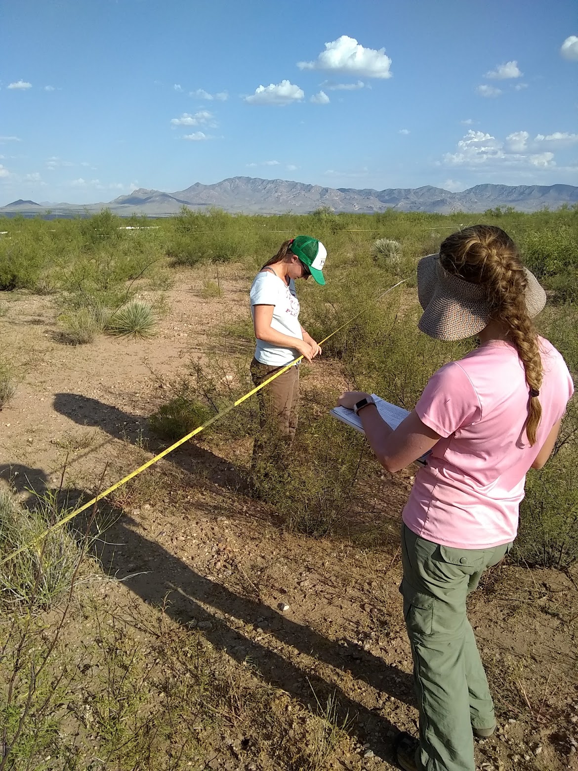
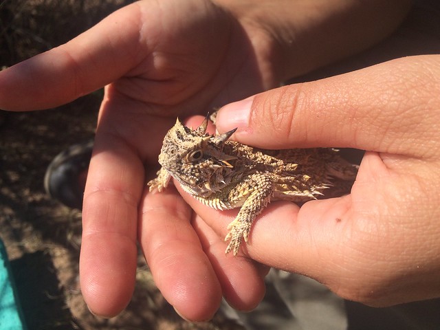
A male K-rat hiding behind a SWRS intern (©Leigh Nicholson)

 

Jessica S. Dudley | PhD candidate
The University of Sydney