What are the rodents eating?

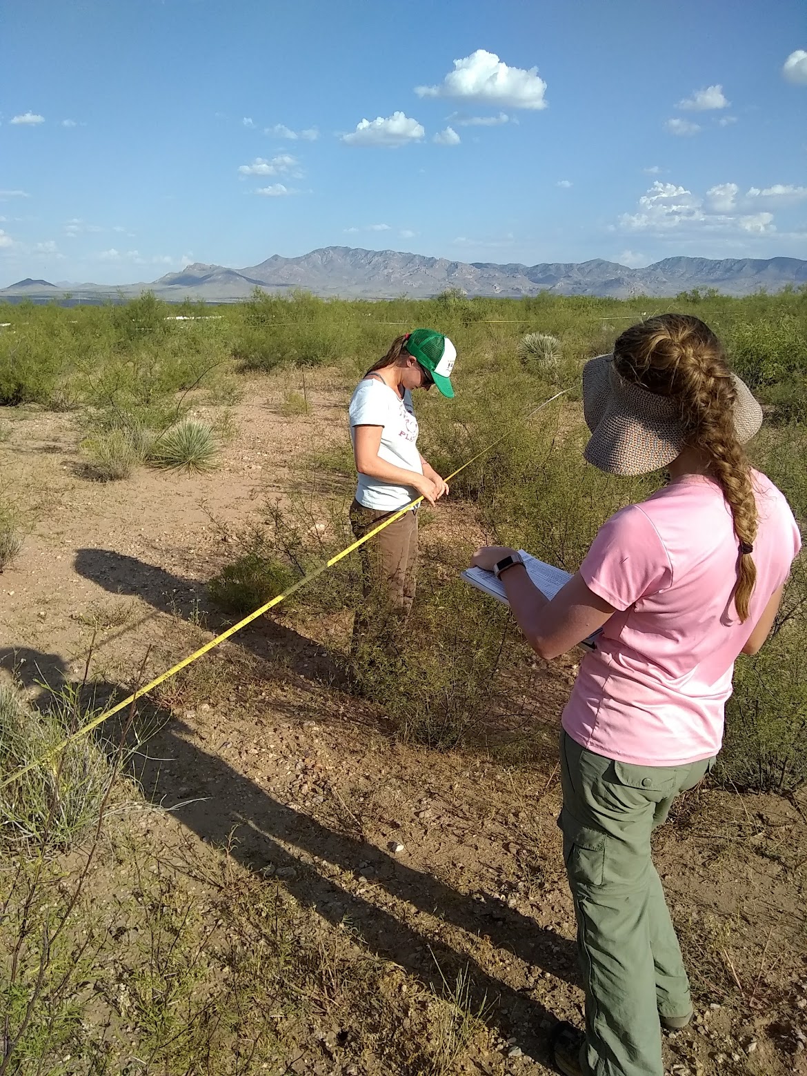
Last week I talked about our adventures in vouchering the plants of Portal. This week I’ll get a little more in depth about the project that prompted this collection push.

This slideshow requires JavaScript.

One of the neatest things about Portal is that we have so many species of rodents coexisting together in the system (up to 21, in fact). Over the years, we’ve speculated on many potential reasons for this. When a fun new technique–DNA metabarcoding–for “easily” analyzing diet from fecal samples popped up on our radar, we started wondering if this was something we could use at our site to ask some neat questions.

For example:

• What are the rodents actually eating?
• Are different species of rodents eating different things? If so, is that possibly one reason so many species are able to coexist at the site?
• Does the presence/absence of a behaviorally dominant species affect the diets of other species?
• How does diet breadth change through time, especially with high seasonal and annual variability in food resources?
• Etc., etc.

Once we started thinking of questions, it was hard to stop. To ask any of these questions, though, we need to know what DNA metabarcoding even meant and whether it could give us the information that we were hoping for. We started looking more into DNA metabarcoding to try to figure out what it actually was, considering none of us have much experience with genetics. We came to understand that, for our intents and purposes, DNA metabarcoding can be best thought of as the simultaneous identification of multiple species from a single sample (fecal samples, in our case). It offers an efficient and effective way to determine diet content without intensive observation or fatal sampling. As it turns out, DNA metabarcoding has actually be around for over a decade, mostly being used in the microbiology world. By the mid-2000s, microbial ecologists had started bringing the technique into ecological circles. Since then, it has been used to enhance biodiversity surveys through environmental DNA, or eDNA, as well as assess the diets of animals. What is just starting to be done with this technique is using it to compare diets between coexisting species.

Figure modified from Valentini et al., 2009

Collecting fecal (and ectoparasite) samples

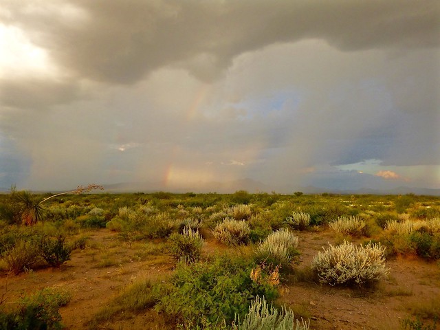
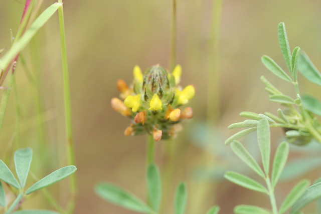
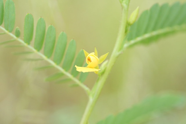
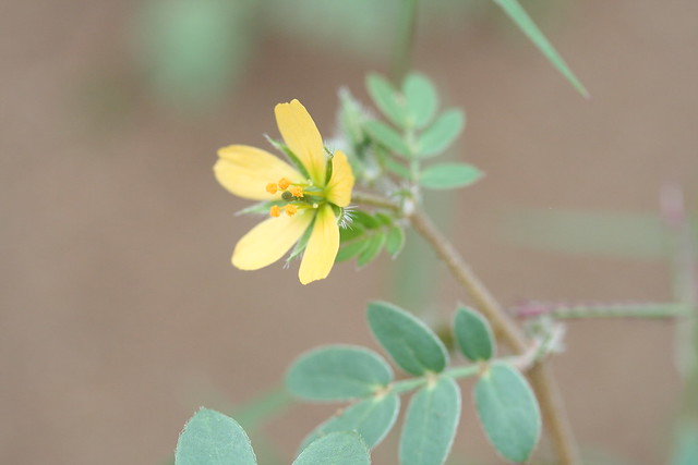
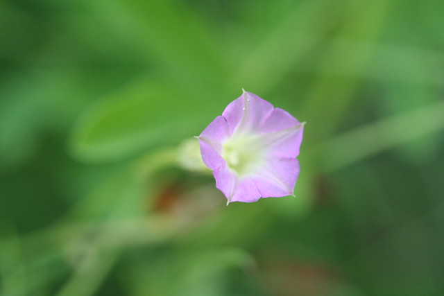
In order to assess the diets, we needed to create a DNA reference library, with DNA from the plants at Portal. This way, we can compare the sequences that are extracted from the rodents’ fecal samples to the plants found at the site. This is where the plant vouchering came into play! We can also pull in data from huge international genetic databases, such as GenBank, to potentially find any plants we’ve missed.

So far, we’ve done four rounds of fecal collections–usually during plant censuses when we have lots of helping hands! Once the fecal samples have gone through the black box of next generation, or high-throughput, DNA sequencing, what we get back is rows upon rows of data about which plants have been eaten by which rodents. While we’re still working through the results, the preliminary data looks promising! We’re able to identify quite a few of the plants that they are eating, and we might even be picking up some shifts in diet between treatment types. Once we have a better picture of what is happening, I’ll chime back in with an update.

Now we can vouch for the plants!

Early on in my dissertation work, I became interested in using a fairly new technique (DNA metabarcoding) to look at what our rodents are eating and if partitioning their diets might be one way so many species exist in our system. I’ll get into more of the details on that project in a subsequent post; for now, though, I want to tell you about a really fun ancillary project. When you’re interested in what the rodents are eating, it’s pretty important to know what they could be eating! Therefore, over the past few plant censuses, we’ve been collecting vouchers and DNA samples for as many of our plant species as we can find!

Having recorded plants at the site for roughly four decades, we are in a pretty fortunate position—we already have a nearly complete list of plants that could be found at the site. Since most of us know more about rodents than plants, however, we wanted to make sure we were correctly identifying our plant species. This requires collecting voucher specimens for every species we come across, pressing them in a plant press, and then dropping them off at the University of Arizona Herbarium for an official verdict from a botanist who specializes in Arizona plants. Once he has looked over our samples and identified them, the herbarium digitizes the specimens. So far, we’ve vouchered about 85% of the nearly 200 recorded plant species at the site.

Quadrats

Identifying plant species

Putting voucher specimens in the plant press

Delivering our precious plants!

Digitized copy of one of our vouchers

For the most part, we’ve been doing a pretty great job identifying our plant species, considering none of us really identify as botanists. We’ve also had some fun surprises along the way, though! For example, for forty years, we thought we had two species of Acacia at the site: 1) whitethorn acacia, Acacia constrica (now Vachellia constricta), and 2) catclaw acacia, Acacia greggii (now Senegalia greggii). As it turns out, however, we’ve probably never had the catclaw acacia at the site! What we’ve been calling A. greggii is actually a species of mimosa, Mimosa aculeaticarpa.

Senegalia greggii

This is not Acacia

This process has also made us more attentive to the plants surrounding us at the site. It was only at the last census that we noticed a large bush/small tree and realized that it was our first (and maybe only) desert willow tree, Chilopsis linearis, at the site. It was hard to believe we’d never noticed one of the biggest plants at the site as being different, but since it was just outside of a plot, there had never really been a reason to notice.

Example of a desert will tree, Chilopsis linearis

We’re looking forward to more surprises in the future, though we still dread having to figure out how to make these changes in the database!

 

Data Analysis with the portalr Package

So you’ve read several posts about the Portal site and have even gone to the official GitHub repo for the data, but it still seems pretty intimidating to handle and do analyses on…

Never fear! The Weecology lab hears your concerns and we are actively working on a software package to smooth out the process. You can check out the project on GitHub.

FAQ

Q: What is it exactly?

A: The portalr project is a software package for the R programming language (http://cran.r-project.org). R is one of the most popular languages for ecology, statistics, and data science; it also has a large open-source community that creates free add-on packages to extend the base functionality.

Q: How do I get the portalr package?

A: There are some basic instructions on the repo page, but in short, the package is still in development and therefore not yet uploaded to CRAN (the comprehensive R archive network). If you are unfamiliar with installing a package from GitHub, the easiest approach is to first install the devtools package, and then use one of its functions to install portalr from GitHub:

install.packages("devtools")
devtools::install_github("weecology/portalr")

Q: What can I do with the package?

A: Several different things! Mainly, it is designed to be a general-purpose interface to the Portal data for R users. It allows you to download the latest iteration of data from the data repo, summarize the data in different ways (e.g. by time, by space, by treatment), and integrate different data sources (e.g. rodents, plants, ants, weather).

Q: That sounds great! How do I get started with that?

A: Well, the package is still under development, but check out the demo below, and feel free to send us comments and suggestions (preferably as an issue here). 👇

Demo

Initial setup

Load in the packages we’re going to use for data manipulation and plotting:

library(tidyverse)
library(cowplot)
library(portalr)

Obtaining the data

To make sure we don’t unnecessarily download the data, we first check whether it might already exist, and if it does, whether the data matches the latest version on the GitHub repo:

# use current folder to store downloaded data
my_path <- "."
rodent_file <- file.path("PortalData", "Rodents", "Portal_rodent.csv")
path_to_rodent_file <- FullPath(rodent_file, my_path)

# check if we already have the latest data
if(!file.exists(path_to_rodent_file) ||
   observations_are_new(base_folder = my_path))
{
  download_observations(base_folder = my_path)
}

Next, we read in the various data tables:

rodent_data_all <- loadData(path = my_path)
print(summary(rodent_data_all))

##                Length Class      Mode
## rodent_data    29     data.frame list
## species_table   8     data.frame list
## trapping_table  6     data.frame list
## newmoons_table  4     data.frame list
## plots_table     4     data.frame list

Rodent Abundances

The first table that we loaded (rodent_data_all$rodent_data) is a record of the observed macrofauna, including rodents, but also other taxa. We first filter the data for missing, unindentified, incomplete, or otherwise erroneous data:

rodent_data_all$rodent_data %>%
  remove_suspect_entries() %>%  
  process_unknownsp(rodent_data_all$species_table, TRUE) %>%
  remove_incomplete_censuses(rodent_data_all$trapping_table, FALSE) %>%
  {.} -> rodent_data

Next, we write a function to summarize the abundances for each species within each sampling trip:

summarize_abundance <- function(rodent_data)
{
return(rodent_data %>%
         mutate(species = factor(species)) %>%
         group_by(period) %>%
         do(data.frame(x = table(.$species))) %>% 
         ungroup() %>%
         select(period, species = x.Var1, abundance = x.Freq)
  )
}
rodent_abundance <- summarize_abundance(rodent_data)

Finally, we want to add the dates of each sampling trip (currently recorded as an index in the period column), as well as the scientific names for each species (currently recorded as a two-letter species code in the species column):

join_census_date <- function(rodent_abundance, newmoons_table)
{
  return(rodent_abundance %>%
           left_join(select(newmoons_table, "period", "censusdate"),
                     by = "period") %>%
           mutate(census_date = as.Date(censusdate))
  )
}
join_scientific_name <- function(rodent_abundance, species_table)
{
  return(rodent_abundance %>%
           left_join(select(species_table, "species", "scientificname"), 
                     by = "species") %>%
           rename(scientific_name = scientificname)
  )
}

rodent_abundance %>%
  join_census_date(rodent_data_all$newmoons_table) %>%
  join_scientific_name(rodent_data_all$species_table) %>%
  select(census_date, scientific_name, abundance) %>%
  {.} -> rodent_abundance

print(summary(rodent_abundance))

## census_date                        scientific_name   abundance      
## Min.   :1977-07-16   Baiomys taylori         : 438   Min.   :  0.000  
## 1st Qu.:1987-05-28   Chaetodipus baileyi     : 438   1st Qu.:  0.000  
## Median :1996-06-02   Chaetodipus hispidus    : 438   Median :  0.000  
## Mean   :1997-03-06   Chaetodipus intermedius : 438   Mean   :  6.273  
## 3rd Qu.:2007-06-16   Chaetodipus penicillatus: 438   3rd Qu.:  5.000  
## Max.   :2017-11-18   (Other)                 :7008   Max.   :285.000  
##                      NA's                    : 438

Plot

Finally, let’s create our plot of species abundances over time:

my_plot <- ggplot(rodent_abundance, 
                  aes(x = census_date, y = abundance)) + 
  geom_line() + 
  facet_wrap(~scientific_name, scales = "free_y", ncol = 3) + 
  xlab("Date") + 
  ylab("Abundance") + 
  scale_x_date(breaks = seq(as.Date("1977-01-01"), 
               to = as.Date("2018-01-01"), "+5 years"), 
  date_labels = "%Y", 
  limits = as.Date(c("1977-01-01", "2018-01-01"))) + 
  theme_cowplot() + 
  theme(axis.text.x = element_text(angle = 90, hjust = 1, vjust = 0.5), 
        legend.position = "bottom", legend.justification = "center", 
        strip.text.x = element_text(size = 10))

print(my_plot)

Conclusion

So that was just one way of viewing the rodent abundance data, but we plan to include many such examples with the `portalr` package. Our goal is to help everyone get up to speed quickly with doing various analyses with the package, and to be able to use all of the different data sources effectively. Again if you have questions or suggestions, please feel free to drop us a line at the GitHub issues page.

The Portal Weather Station

For the history of the project, weather monitoring has always accompanied the collection of rodent, plant, and ant data. At first, this was done manually. Portalites from 1980 to 1989 measured rain in a rain gauge, and used something called a hygrothermograph to measure temperature and humidity.

Hygrothermograph

Then things started to get fancy. In 1989, an automated weather station was installed. This is the desert though, and leaving expensive toys out in the rain, dust and lightning takes it’s toll.

At least the lightning storms leave us with some nice scenery after they try to blow up our weather station.

All things considered, our weather stations have stood up pretty well. The first lasted from 1989 until 2002. And the station from 2002 is still limping along, although it’s had its moments (it tends to have a bit of a tantrum after being struck by lightning). We connected to the dataloggers for those stations directly. That is, as part of their monthly duties, the rodent RA has to connect to the datalogger, download the data, and bring it back to the lab for checking and appending to the database.

2002 station with temperature and humidity sensor, and rain gauge (right)

Sarah connecting to the 2002 datalogger

Anticipating the 2002 station’s impending demise, in August 2016 we upgraded to a new station, and took the opportunity to make some improvements.

The majestic new station

Of course we continue to collect data on precipitation, temperature and humidity. But we’ve also gotten to add a wind sensor (wind speed and direction), pyranometer (solar radiation), and barometer (atmospheric pressure). Having these additional data means that we can also calculate things like evapotranspiration, sunshine hours, and windchill. We have also added a new program to collect fine-scale precipitation data during storms. When a precipitation event begins, the datalogger begins recording total precipitation every 5 minutes until the storm ends.

The addition of a cellular modem is another major improvement. Rather than downloading it monthly in the field, we access the data remotely. The data trickle in to  our data repo whenever edits are made to trigger a new build, or at least once a week, and quality control happens automatically. Our station has a Wunderground account (from whence the fancy little widget in the sidebar comes). And we’ve mounted the phenocam (featured in an earlier post, and another widget in the sidebar) to it.

Aside from just being darn cool, the upgrades have improved our data collection. We can see what the weather has been at our exact location at any time. That means we can know what to expect from the plants before we go for a census (as much as that’s possible). And we can communicate with the datalogger at anytime. If something is wrong with the weather station, we’ll know immediately. It may be possible to fix the problem remotely. If not, the rodent RA can plan to fix it while she’s down there, instead of discovering the problem at the site, waiting until the next month to fix it, and losing at least a month worth of data. And we can always send new programs to the datalogger, if we want to add new data tables make improvements.

Find our weather data, updated sub-weekly, on the Portal Data github repository.

A Vegetation History

My Portal story begins in 1991 when Jim Brown offered me the opportunity to be the Portal postdoc. Among other things, this meant I organized the yearly ant census in which we spent about 2 weeks counting the abundance of ant colonies on the experimental plots. In one of my first summers, I hired Don Sias to help with the census. Don was a non-traditional student and had previously traveled extensively throughout the southwest. One day he mentioned to me that the vegetation in the San Simon valley looked pretty “beat up”. By that he meant the vegetation, dominated by shrubs, had the look of a grassland that had become desertified.

I was intrigued by Don’s comment for two reasons. First, Brown and Heske (1990) had recently described a significant increase in grass cover on Portal plots that removed kangaroo rats and mentioned that the site was “near the zone of natural transition from desert to grassland”. Second, while desertification is often associated with overgrazing, Heske and Campbell (1991) found no difference in vegetation across the Portal grazing fence despite 11 years of livestock removal – why hadn’t the grasses recovered with livestock removal if the site had once been a grassland?

When I returned to Albuquerque, I recall asking Jim about the vegetation history of the site. He said that he wasn’t sure and encouraged me to see what I could figure out. That led me to the U.S. General Land Office Surveyors notes. The surveyors described the dominant vegetation they traveled through as each mile-long section line was surveyed. Many, but not all, of the lines near our site were surveyed between 1875 and 1883 and the most common description was “good grass”. However, when the surveyors came back to complete their work in the early part of the 20th century, the descriptions were dominated by the words “scattered shrubs” while grass was not mentioned at all. This change in vegetation coincided with large introductions of livestock into the San Simon valley in the late 1880’s, and then a major drought in the early 1890’s that resulted in tremendous livestock mortality due to starvation.

Our understanding of the recent vegetation change at the site can help to explain the observed shifts in grass cover observed at Portal both over time and across the rodent treatments. It also prompted further investigations into desertification and the role of livestock in affecting soil compaction as a mechanism that helps to explain why reversals of desertification (a recovery of perennial grasses) can require several decades. Finally, it illustrates how careful observations by students and researchers that visit the site can lead to interesting questions and new discoveries.

This slideshow requires JavaScript.

I’ve been very fortunate to have worked on the Portal system for almost 30 years. Change seems to be the constant at Portal – you never know what you’ll see and how things have changed since the last visit. This complex system continues to be a source of inspiration as we try to understand it (or, as Morgan says, “unravel her mysteries”).

Portal: Then and Now

A lot can change in 40 years.  This is perhaps never more apparent than when you find a box of old photographs, and start comparing then to now.  When the Weecology lab immigrated from Utah to Florida in 2015, just such a box surfaced: a glimpse back in time to the beginning of the portal project.  I did my best to re-create some of these photographs—trying to line up horizons and mountains—to show how the site has changed over 40 years.

One thing is immediately apparent: the shrubs have grown up.  The left side of these photographs were taken in 1977 (photographer unknown), and the right side in 2015 (photographer Erica Christensen).  What happened to the rows upon rows of aluminum flashing, indicating the location of the rodent fences?  I assure you the fences are still there, they’re just obscured by the jungle.

This slideshow requires JavaScript.

The fact that you used to be able to see clear across the site is shocking to the modern research assistants. These days, part of the training for new RAs taking over work at Portal is receiving a map from the previous RA with routes drawn in for the best paths between plots. Navigation is not trivial.

Erica, circa 2012, demonstrating the problem (photographer Sarah Supp)

Other locations at the site don’t look too different from how they looked in the ‘70s. Grass cover comes and goes depending on the strength and timing of monsoon rains every year, but some plots don’t seem as affected as others by the shrub explosion.

This slideshow requires JavaScript.

While shrub encroachment is an annoying obstacle to a human, it is a major ecological shift to a rodent. This was the topic of a 1997 paper by Brown, Valone, and Curtin, where they found a 3-fold increase in shrub cover between 1980 and 1995 by analyzing historical aerial photographs. The authors also noted a concurrent decline in rodent species affiliated with arid grassland (banner-tail kangaroo rat and silky pocket mouse) and an increase in species affiliated with arid shrubland (desert pocket mouse and Bailey’s pocket mouse). It looked like the grassland species were on their way out and the shrubland species were taking over. However banner-tails and silkys continue to be found at the site, despite the fact that shrub cover has increased, if anything, since 1995. They’re now quite rare; these days we pretty much only see them when the rains align just right to give us a “grassy year.”

Nobody tell this adorable silky pocket mouse we’re a shrub habitat now

Those of us who have worked at Portal know that things are always different every time you go down, and yet some things never change. Which is why we keep going, keep collecting data: even after 40 years there is still a lot to learn.

Reference:
Brown, J.H., Valone, T.J., and Curtin, C.G. (1997). Reorganization of an arid ecosystem in response to recent climate change. Proc. Natl. Acad. Sci. 94, 9729–9733.

2017 Summer Plant Census

Twice a year the Portal crew gets a little larger, and spends a few extra days, and we count plants on all 384 quadrats. Despite some of us being in our second decade of visiting the site, and everyone on the plant crew being intimately familiar with most of the species at the site, and that the rodent RA has been watching the plants grow and giving us monthly updates, we still never really know what we’re going to find once we get out there. The desert does what it wants.

The uncertainty seems especially high for the summer plant community. Some years we arrive to an ocean of grass, waving in the breeze. Those are the years we spend a lot of ‘quality time’ with each quadrat. Other years we arrive to a dustbowl. We walk around the site laying our PVC quadrat down and picking it back up again and saying ‘zero’ 384 times. [Okay, we don’t really ever get all zeros. But it feels like that when you’re out there.] And some years we show up to find some new arrivals, species that finally decided to show up after 40 years. Then we spend less time counting individual blades of grass, and more time pouring over our regional species list and plant ID guides.

Summer 2014, Morgan, Tom and Erica counting Aristida adscensionis and Bouteloua aristidoides, a lot of it

Summer 2015, ‘Who are you and where did you come from?’

 

This summer was pretty good for forb diversity. Forb species like Dalea, Cassia, Kallstroemia, Ipomea and Sida were relatively abundant.

In the summer we also measure shrub cover on the plots, so we get some bonus quality time with the plants.

 

There are lots of other bonuses to the summer plant census that make up for the brain-melting heat. As we’re walking around the plots, we get to see snakes (Mojave rattler, Common king snake, gopher snake, coachwhip, and Coral snake on this trip), horned lizards, turtles, tarantulas and exceptional insect diversity that are not out and about from October to May.

And there’s nothing like a Portal monsoon sunset.

Ode to six-legged wonder

If four legs are great, six legs are better. Right? For forty years now, the Portal Project has primarily focused on two-legged creatures trapping, studying, and sometimes cuddling small, furry four-legged creatures. But we haven’t ignored the six-legged inhabitants of our long-term research site, and I am going to tell you more about them now.

Which one of these is least like the other?

I am the Ernest lab entomologist, who doesn’t consider herself an entomologist. I am interested in biodiversity, community, and macroecological patterns like those studied by generations of Portal rodent researchers. I just happen to study them using bees. There are over twenty thousand species of bees in the world, and about four thousand in North America. My research so far has focused on the community ecology of native bees in a global hotspot of bee diversity in California. But as fate or luck would have it, another documented haven for native bees lies just down the road from our long-term rodent site in Portal. Between 2000 and 2007, bee researcher Robert Minckley documented 383 different species and 69 genera of bees from the San Bernardino Valley of Arizona and Mexico. The Smithsonian’s Southwestern Research Station, which is nestled up in the hills only a few miles from our rodent site, also celebrates the insect diversity of this area with field courses focused on bees or ants that attract dozens of eager entomologists from all around the world every summer.

Look familiar? This is the San Bernardino Valley on the border of Arizona and Mexico, just 50 miles south of our Portal research site. By BAlvarius – Own work, CC BY-SA 3.0, https://commons.wikimedia.org/w/index.php?curid=11806210

A few months ago, I set out to see what kind of six-legged creatures we have scurrying around at Portal. My adventurous and ever-curious lab mates were willing to help, and (I think) even had a bit of fun learning to collect, pin, and curate bugs. During the March and May 2017 rodent censuses, we used a variety of passive (let the insects come to the trap) and active (go get ’em!) methods of insect collection to sample the local diversity on six legs:

• Pan traps are brightly colored bowls full of soapy water that (passively) attract flying insects like bees that visit the bowls, fall into the water, and can be strained out and examined later.
• Aerial nets (or “butterfly nets”) can be used to actively snag insects flying by or foraging on flowers, or can be used to more methodically sweep the ground to sample insects hiding in the grass or shrubs.
• Blacklights lit underneath a white sheet at night passively bring in moths, roaches, and other nocturnal creatures that are drawn to ultraviolet wavelengths, perhaps because they confuse them with the moonlight they use to navigate, and can be scooped into collecting vials from their perches on the sheet.
• Pitfall traps are plastic containers that are buried in the ground with their top openings flush with the ground level and covered with a coarse mesh with a hole in the center. Insects walking along the ground cross the mesh, fall into the hole, and are preserved in a small amount of ethanol at the bottom of the container. Do you think this is active or passive insect collecting? (Hint: we leave them out all day and only come back at dusk to check what is there.)
• The crowd favorite was probably the “beat sheet,” which is simply a white sheet placed on the ground underneath an intriguing shrub, which is then vigorously beat with a piece of PVC pipe, a shovel, a hockey stick — really any bludgeoning tool will work. Insects that fall onto the sheet are then sucked up into an aspirator device — like a tiny, scientific, human-powered vacuum — and transferred into a collecting vial. This method of collecting is pretty active!

Erica and Ellen getting cozy with the shrub they are about to beat.

Pitfall trap, ready to go.

All smiles discovering the contents of their pan traps.

Glenda and Kristina would never really drink ethanol.

The spoils of our collecting efforts were creepy, crawly, and diverse.  The field crew had fun learning to pin them using the cooler and truck tailgate as our insect lab. Then I mailed them back to the lab and have been working on labeling, curating, and identifying our new Portal insect collection.

Then just last week I took them to campus for a photo glam session with the fancy microscope camera. Take a look:

This slideshow requires JavaScript.

I’m certainly not the only one who has been interested in the insect fauna in and around the rodent plots at Portal. Ants were actually a big part of the original research design. Between 1977 and 2009, ant colonies were censused once a year at every stake on all the plots, and between 1988 and 2009 ants were also baited (with Pecan Sandies!) and counted at 25 stakes in the thirteen unmanipulated plots. Research papers using this data, which is available to the public on the Weecology GitHub PortalData repository, have been authored by Tom Valone, Mike Kaspari, and more. Other brilliant ecologists like Deborah Gordon and Nate Sanders have also studied ant diversity, behavior, and community composition in the valley around our research site. I was actually following some of these researchers’ work long ago when I was first looking for graduate advisers and nerding out over my giant book about ants. And now here I am, working with the rodent branch of the legendary Portal Project while focusing on bees for my own work. It’s a small world after all, full of small six-legged wonder.

 

Learn more by checking out some of the published science on the ecological entomology around Portal:

Gordon, Deborah M. 1999. Ants at work: how an insect society is organized. Simon and Schuster.

Davidson, D.W., Inouye, R.S., Brown, J.H. 1984. Granivory in a Desert Ecosystem: Experimental Evidence for Indirect Facilitation of Ants by Rodents. Ecology, 65(6), 1780-1786.

Kaspari, M., & Valone, T. J. 2002. On ectotherm abundance in a seasonal environment—studies of a desert ant assemblage. Ecology, 83(11), 2991-2996.

Minckley, R. 2008. Faunal composition and species richness differences of bees (Hymenoptera: Apiformes) from two north American regions. Apidologie. 39: 176–188.

Sanders, Nathan J., and Deborah M. Gordon. 2003. Resource‐dependent interactions and the organization of desert ant communities.” Ecology 84.4: 1024-1031.

Sanders, N. J., & Gordon, D. M. 2000. The effects of interspecific interactions on resource use and behavior in a desert ant. Oecologia, 125(3), 436-443.

Valone, T. J., & Kaspari, M. 2005. Interactions between granivorous and omnivorous ants in a desert grassland: results from a long‐term experiment. Ecological Entomology, 30(1), 116-121.

 

This four-legged creature thinks Portal is just the best place she’s ever been.

 

 

Portal Phenocam

You may have noticed the super-cool daily images featured in last week’s post. They’re from our new network camera.

For starters, it allows us to do things like watch our desert field site turn from brown to green in no time flat (and back to brown again this winter).

 

 

 

 

But even cooler, our camera is part of the PhenoCam Network. They’re organizing a network of near-surface remote sensing images from sites all over the world. This creates a time series of images, in RGB and infrared, that can be used for phenology monitoring by the PhenoCam folks, us, or anyone who’s interested.

 

 

 

 

The PhenoCam folks make all the imagery freely available to download. From installation and configuration to image analysis, they provide awesome support. And their R package phenopix provides a quickstart to using phenocam imagery.

Pregnancy in Kangaroo rats

~While everyone’s busy at ESA this week, we’d like to keep the 40th anniversary ball rolling with a guest post from a visiting researcher at Portal. Jess Dudley has been using the Portal area to compare pregnancy in kangaroo rats and Australian marsupials. We’ll be featuring other guest posts through the rest of the year. (If you’d like to do something similar, please send us your info!)~

 

In July 2015 I travelled the 24+ hours from Sydney, Australia to the beautiful town of Portal to research pregnancy in Kangaroo rats. To everyone’s astonishment we do not have Kangaroo rats in Australia! I am sure I don’t need to explain my fascination with Kangaroo rats with this audience but in terms of pregnancy they have some unique features which differ from most rodents. This finding by King and Tibbitts in the 1960’s led me to wonder how the placenta forms during pregnancy in these resilient animals. To answer these questions I was lucky enough to visit Portal twice in the summers of 2015 and 2017 to trap Kangaroo rats and collect tissue from the females. I have completed Transmission and Scanning Electron Microscopy as well as Western blotting and Immunofluorescence microscopy on the uterine samples from pregnant Merrriam’s kangaroo rats to determine what structural and molecular changes are needed for implantation of the early embryo and ultimately a successful pregnancy.

Fat tailed dunnart (Sminthopsis crassicaudata) (https://museumvictoria.com.au)

 

My initial research into the molecular mechanisms of implantation and pregnancy began in an Australian marsupial species the Fat tailed dunnart (Sminthopsis crassicaudata) which has the same partly invasive placenta as the Kangaroo rat.

Fat tailed dunnart (Sminthopsis crassicaudata) (https://museumvictoria.com.au) range. IUCN (International Union for Conservation of Nature) 2016.

 

Through these comparative studies we have found that the molecular mechanisms allowing for successful pregnancy are conserved among eutherian and marsupial mammals during the early stages of pregnancy regardless of how invasive their placenta becomes.

An Immunofluorescence image showing localization of adhesion molecules in green and cell nuclei in blue from a non-pregnant Merriams’ Kangaroo rat. Uterine Epithelial Cells = UEC. Lumen = L.

Transmission Electron Microscopy image of uterine epithelial cells from a Merriams’ Kangaroo rat in the
early stages of pregnancy.

It has been an amazing experience to work in the Chihuahuan Desert. I was introduced to animals that I had never heard of and witnessed countless stunning sunrises and sunsets as well as beautiful starry night skies. It was an experience I will never forget. I would like to thank Glenda Yenni, Leigh Nicholson and all of the wonderful people at the Southwestern Research Station for their assistance and advice during the completion of this project.

A male K-rat hiding behind a SWRS intern (©Leigh Nicholson)

 

Jessica S. Dudley | PhD candidate
The University of Sydney